Data preparation for analysis is made possible by data scientists thanks in part to data processing in R. In order to allow for reliable analysis, raw data must typically be cleaned and modified to remove missing values, outliers, and other anomalies.
In my previous article, I had gone through an overview of how the RStudio IDE looks like and the features it provides. And in this post, we will take a look at how there are packages in R, such tidyr and dplyr, which make it simple to clean and transform data.
The ability for data scientists to swiftly extract insights from data is another reason why data manipulation is crucial in R. For instance, a data scientist can use R to classify the data by location, determine the average sales, and display the results if they need to assess how a product performs in various geographic areas.
R has a number of visualisation packages, such ggplot2, that make it simple to plot and map in order to convey ideas easily.
Finally, the ability to manipulate data in R is essential for data scientists to automate tedious procedures. Data scientists may efficiently perform challenging data manipulation tasks, such merging datasets, without having to perform them manually by developing R scripts.
Table of Contents
Introduction to Data Manipulation with R
Data manipulation is a critical step in data science, and R provides a rich set of tools for working with data. Here’s an introduction to data manipulation with R, including importing and exporting data:
- Importing Data: CSV, Excel, and text files are just a few of the file types that R can read data from. To read data from a CSV file, use the read.csv() method; to read data from an Excel file, use the read excel() function. Data from a text file can be read using the read.table() function.
- Exporting Data: R also offers data export to a number of file types. As opposed to the write.xlsx() method, which is used to write data to an Excel file, the write.csv() function writes data to a CSV file. Data is written to a text file using the write.table() function.
- Data Types: R handles a variety of data types, including logical, character, factor, and numeric. Understanding data types is essential for manipulating data since various operations behave differently when applied to various data types.
- Data Frames: One of the most common data structures in R is the data frame. They are used to store data in rows and columns and are comparable to database tables. A data frame is constructed using the data.frame() function.
- Subsetting: Selecting a subset of rows or columns from a data frame is the process of subsetting. The bracket notation ([]) is used to subset columns, while the subset() function is used to subset rows based on a logical condition.
- Joining: The process of joining involves integrating two or more data frames based on a shared variable. Two data frames are joined using the merge() function based on a common variable.
- Reshaping: Data transformation from one format to another is called reshaping. Data can be transformed from a wide format to a long format and vice versa using the reshape() method.
Usage of the 'dplyr' Package to Manipulate Data

The dplyr package is a powerful tool for data manipulation in R. It provides a set of functions that make it easy to perform common data manipulation tasks such as filtering, selecting, and aggregating data. Here’s a brief introduction to using the dplyr package to manipulate data:
- Installing the dplyr package: You must separately install the dplyr package using the install.packages() function because it is not part of the default R installation.
- Loading the dplyr package: After installing the package, you will need to load it into your R session using the library() function.
- The five main dplyr functions: The dplyr package provides five main functions for data manipulation: filter(), select(), arrange(), mutate(), and summarize(). Here’s a brief overview of what each function does:
- filter( ) : Using this function, rows can be chosen based on a logical condition. The filter() function, for instance, can be used to pick all rows where a variable exceeds a specific value.
- select( ) : To choose columns from a data frame, use this function. For instance, you can choose only the columns in which you are interested by using the select() function.
- arrange( ) : Using this function, rows can be sorted according to one or more variables. The arrange() function, for instance, can be used to order a data frame according to a name or a date.
- mutate( ) : Using the mutate() function, one can transform existing variables to produce new ones. For instance, you can compute a new variable based on an existing variable using the mutate() function.
- summarise( ) : With the help of the summarise() function, you may compute summary statistics for one or more variables. For instance, you can get a variable’s mean or median using the summarise() method.
Here’s an example of how to use the dplyr package to filter, select, and arrange data:
					r
library(dplyr)

# Load data
data <- read.csv("data.csv")

# Select and filter data
filtered_data <- data %>%
  select(name, age, gender) %>%
  filter(age > 30, gender == "female") %>%
  arrange(name)

# Print filtered data
print(filtered_data)
Next, the information is organised alphabetically by name. The resulting data frame is then printed to the terminal.
Learning to use the dplyr package, a potent tool for R data processing, can significantly increase your productivity and effectiveness as a data scientist.
Cleaning and Preprocessing Data using 'tidyverse'
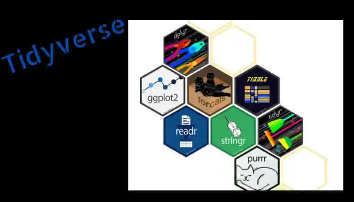
Data preparation and cleaning are crucial phases in data analysis. R’s ‘tidyverse’ package offers a selection of tools for cleaning and preprocessing data. In this post, we’ll explore the processing of data using the tidyverse package.
- Installing the tidyverse package: You must separately install the tidyverse package using the install.packages() function because it is not part of the standard R installation.
- Loading the tidyverse package: You must use the library() method to load the package into your R session after installing it.
- Importing the data: You must first import the data into R in order to clean and preprocess it. Several functions for importing data are available in the tidyverse package, including read_csv(), read_excel(), and read_table().
These functions can import data from a number of file types, including text files, Excel, and CSV. - Data cleaning with tidyr: The tidyr package provides tools for cleaning and reshaping data. Some of the functions provided by tidyr include:
- gather( ) : This function is used to reshape data from wide to long format.
- spread( ) : This function is used to reshape data from long to wide format.
- separate( ) : This function is used to split a column into multiple columns.
- unite( ) : This function is used to combine multiple columns into a single column.
- Data cleaning with dplyr: The dplyr package provides tools for filtering, selecting, arranging, and summarizing data. Some of the functions provided by dplyr include:
- filter( ) : This function is used to select rows based on a logical condition.
- select( ) : This function is used to select columns from a data frame.
- arrange( ) : This function is used to sort rows based on one or more variables.
- mutate( ) : This function is used to create new variables by transforming existing variables.
- summarize( ) : This function is used to calculate summary statistics for one or more variables.
- Handling missing data: The tidyr and dplyr packages also provide functions for handling missing data. Some of these functions include:
- na_if( ) :This function is used to replace specific values with missing values.
- drop_na( ) : This function is used to remove rows with missing values.
- fill( ) : This function is used to fill missing values with a specified value.
- The process of scaling numerical data so that it falls inside a predetermined range is known as normalization. Data can be normalised using the base R installation’s scale() function.
					r
library(tidyverse)

# Import data
data <- read_csv("data.csv")

# Reshape data
tidy_data <- data %>%
  gather(variable, value, -id) %>%
  separate(variable, into = c("variable1", "variable2"), sep = "_") %>%
  spread(variable2, value) %>%
  unite(new_variable, variable1, variable2)

# Filter and select data
clean_data <- tidy_data %>%
  filter(variable1 == "age", !is.na(new_variable)) %>%
  select(id, new_variable)

# Normalize data
normalized_data <- clean_data %>%
  mutate(new_variable = scale(new_variable))

# Export data
write_csv(normalized_data, "clean_data.csv")
In this example, we import data from a CSV file and then reshape, filter, and select the data using the tidyr and dplyr packages. The data is then normalised using the scale() method before being exported to a fresh CSV file. Now that the data has been cleaned, it may be analyzed further.
Why is Data Wrangling necessary for applications in Data Science?
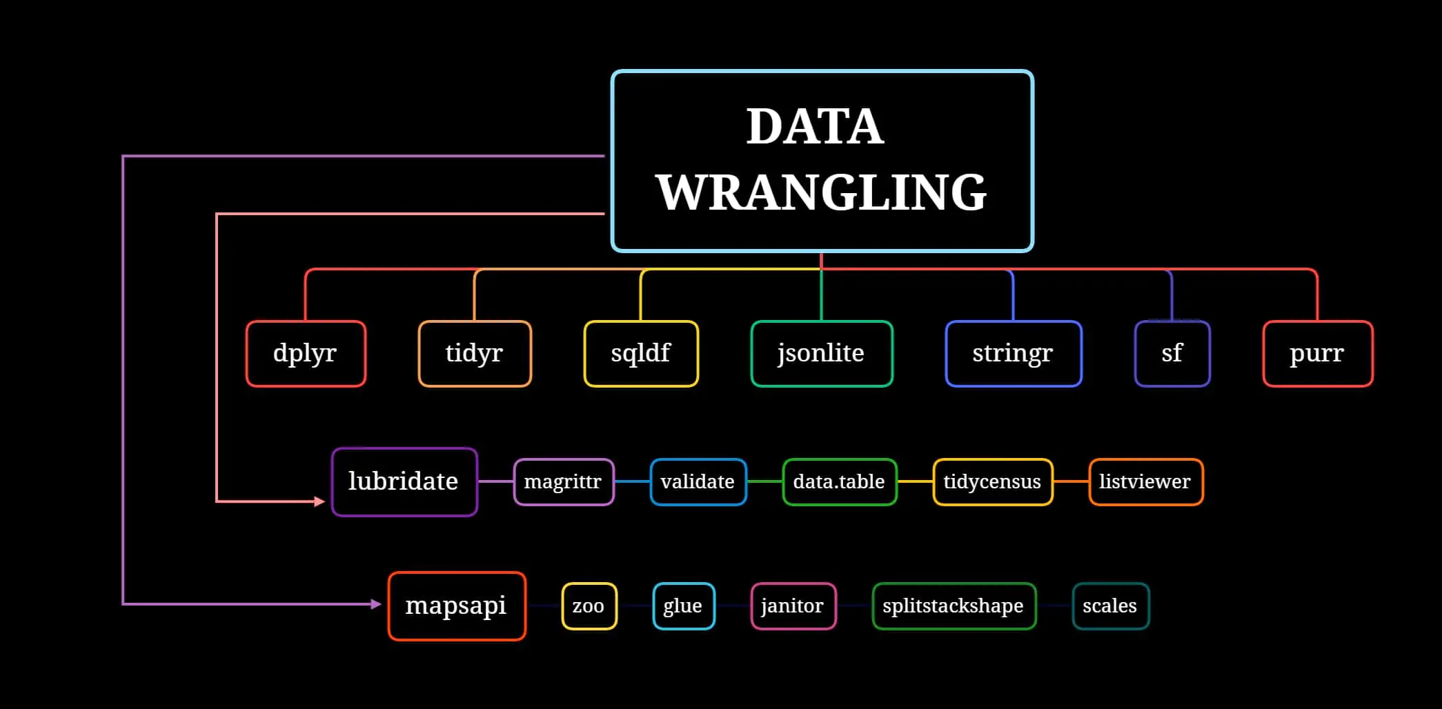
Identifying missing values, outliers, and other anomalies that must be fixed before analysis can also be done with the use of this technique. As a result, preprocessed data can yield more precise and credible research, better insights, and more well-informed choices.
Therefore, it is crucial to take the time and effort necessary to clean and prepare data before using it for data science applications.
In data science, data processing is a time-consuming and typically painful process. The advantages of doing so, however, are enormous. It can result in more accurate predictions and insights, which is a key advantage. The analysis is based on a more dependable and consistent dataset after the data has been wrangled or “munged”. As a result, the forecasts and insights that are generated are probably more accurate and useful.
The ability to identify patterns and relationships that might otherwise go undiscovered is another advantage of preparing data. Data scientists can standardize the data, eliminate extraneous information, and detect missing values or outliers through this technique. This can serve to illustrate trends or patterns that might not have been visible otherwise, leading to fresh observations and discoveries.
With the help of R’s visualisation utilities, like ggplot2, it is simple to plot and map data in order to clearly communicate concepts.
The security and privacy of data are also improved through this step. Preprocessed data often lowers the possibility of sharing or exposing private or sensitive information. As data scientists may make sure that the data is secure to use and that privacy is respected by deleting personally identifying information and other sensitive data points.
All this, in addition to making well-informed business decisions – makes the whole process of data transformation fundamental for successful data science projects.